This post covers the workflowsets package, which focuses on quickly and easily fitting a large number of models by creating a set that holds several workflow objects.
Setup
Packages
The following packages are required:
Data
I utilized the penguins data set from the modeldata package for these examples.
Note that the outcome variable is forced to be binary by assigning all the odd-numbered rows as “Chinstrap” and the even numbered rows as “Adelie”. This is done to (1) ensure that the outcome is binary so certain functions and techniques can be used and (2) make the outcome a little more difficult to predict to better demonstrate the difference in the construction of the modeling algorithms used. In addition, rows with missing values are removed.
Code
data("penguins", package = "modeldata")

penguins_tbl <- penguins %>%
  mutate(
    #> Need a binary outcome
    species = ifelse(row_number() %% 2 == 0, "Adelie", "Chinstrap"),
    species = factor(species, levels = c("Adelie", "Chinstrap"))
  ) %>%
  filter(!if_any(everything(), \(x) is.na(x)))

penguins_tbl %>%
  count(species)
# A tibble: 2 × 2
species n
<fct> <int>
1 Adelie 167
2 Chinstrap 166Model Preparation Process
As discussed in a previous post in this series, some preparation work is required before constructing a workflow(), and by extension a workflow_set(). As before, these steps follow the tidymodels process.
Data Splitting
Referencing a previous post on the rsample package, a 70/30 train/test initial_split() on both data sets is taken. It is then passed to the training() and testing() functions to extract the training and testing data sets, respectively.
set.seed(1914)
penguins_split_obj <- initial_split(penguins_tbl, prop = 0.7)penguins_train_tbl <- training(penguins_split_obj)
penguins_train_tbl# A tibble: 233 × 7
species island bill_length_mm bill_depth_mm flipper_length_mm body_mass_g
<fct> <fct> <dbl> <dbl> <int> <int>
1 Chinstrap Biscoe 36.4 17.1 184 2850
2 Adelie Biscoe 52.1 17 230 5550
3 Adelie Dream 50.8 18.5 201 4450
4 Adelie Dream 37.2 18.1 178 3900
5 Chinstrap Biscoe 45.5 14.5 212 4750
6 Chinstrap Biscoe 39 17.5 186 3550
7 Chinstrap Biscoe 48.2 15.6 221 5100
8 Adelie Dream 52 19 197 4150
9 Chinstrap Biscoe 45.4 14.6 211 4800
10 Chinstrap Biscoe 38.1 17 181 3175
# ℹ 223 more rows
# ℹ 1 more variable: sex <fct>penguins_test_tbl <- testing(penguins_split_obj)
penguins_test_tbl# A tibble: 100 × 7
species island bill_length_mm bill_depth_mm flipper_length_mm body_mass_g
<fct> <fct> <dbl> <dbl> <int> <int>
1 Chinstrap Torgers… 40.3 18 195 3250
2 Adelie Torgers… 39.2 19.6 195 4675
3 Chinstrap Torgers… 38.7 19 195 3450
4 Adelie Torgers… 46 21.5 194 4200
5 Chinstrap Biscoe 37.8 18.3 174 3400
6 Adelie Biscoe 37.7 18.7 180 3600
7 Adelie Biscoe 38.2 18.1 185 3950
8 Chinstrap Biscoe 40.6 18.6 183 3550
9 Chinstrap Dream 36.4 17 195 3325
10 Adelie Dream 42.2 18.5 180 3550
# ℹ 90 more rows
# ℹ 1 more variable: sex <fct>Data Processing
Referencing another previous post on the recipes package, pre-processing steps are performed on the training data set. The resulting recipe() object is then passed to the prep() function to prepare it for use. The result is then passed to the juice() function to extract the transformed training data set.
Note that a slightly different method is used here than in the workflows post. Instead of creating a recipe() for each modeling algorithm, three separate recipes are created without regard to the modeling algorithm. More detail will be provided in a later section, but the short explanation is that each combination of recipe() and modeling algorithm will be used, so there is no reason to specify which recipe() goes with which modeling algorithm.
This recipe() contains just the model formula and the training data set. This may seem needless, as passing this recipe() to the juice() function just returns the original data set. This is what is desired, however, and using recipe() objects makes working with a workflow() easier (in my opinion).
# A tibble: 233 × 7
   island bill_length_mm bill_depth_mm flipper_length_mm body_mass_g sex
   <fct>           <dbl>         <dbl>             <int>       <int> <fct>
 1 Biscoe           36.4          17.1               184        2850 female
 2 Biscoe           52.1          17                 230        5550 male
 3 Dream            50.8          18.5               201        4450 male
 4 Dream            37.2          18.1               178        3900 male
 5 Biscoe           45.5          14.5               212        4750 female
 6 Biscoe           39            17.5               186        3550 female
 7 Biscoe           48.2          15.6               221        5100 male
 8 Dream            52            19                 197        4150 male
 9 Biscoe           45.4          14.6               211        4800 female
10 Biscoe           38.1          17                 181        3175 female
# ℹ 223 more rows
# ℹ 1 more variable: species <fct>
This recipe() adds a step to the previous that one-hot encodes all categorical variables.
recipe_2_obj <- recipe_1_obj %>%
  step_dummy(all_nominal_predictors(), one_hot = TRUE)

recipe_2_obj %>%
  prep() %>%
  juice()
# A tibble: 233 × 10
bill_length_mm bill_depth_mm flipper_length_mm body_mass_g species
<dbl> <dbl> <int> <int> <fct>
1 36.4 17.1 184 2850 Chinstrap
2 52.1 17 230 5550 Adelie
3 50.8 18.5 201 4450 Adelie
4 37.2 18.1 178 3900 Adelie
5 45.5 14.5 212 4750 Chinstrap
6 39 17.5 186 3550 Chinstrap
7 48.2 15.6 221 5100 Chinstrap
8 52 19 197 4150 Adelie
9 45.4 14.6 211 4800 Chinstrap
10 38.1 17 181 3175 Chinstrap
# ℹ 223 more rows
# ℹ 5 more variables: island_Biscoe <dbl>, island_Dream <dbl>,
# island_Torgersen <dbl>, sex_female <dbl>, sex_male <dbl>This recipe() adds a step to the previous that normalizes all continuous variables.
recipe_3_obj <- recipe_2_obj %>%
  step_normalize(all_numeric_predictors())

recipe_3_obj %>%
  prep() %>%
  juice()
# A tibble: 233 × 10
bill_length_mm bill_depth_mm flipper_length_mm body_mass_g species
<dbl> <dbl> <dbl> <dbl> <fct>
1 -1.41 -0.00476 -1.24 -1.72 Chinstrap
2 1.37 -0.0552 2.02 1.63 Adelie
3 1.14 0.701 -0.0360 0.266 Adelie
4 -1.26 0.499 -1.67 -0.415 Adelie
5 0.204 -1.32 0.745 0.637 Chinstrap
6 -0.945 0.197 -1.10 -0.849 Chinstrap
7 0.682 -0.761 1.38 1.07 Chinstrap
8 1.35 0.953 -0.320 -0.106 Adelie
9 0.186 -1.26 0.674 0.699 Chinstrap
10 -1.10 -0.0552 -1.46 -1.31 Chinstrap
# ℹ 223 more rows
# ℹ 5 more variables: island_Biscoe <dbl>, island_Dream <dbl>,
# island_Torgersen <dbl>, sex_female <dbl>, sex_male <dbl>Model Specifications
Referencing another previous post on the parsnip package, three model specifications are constructed. The first is a logistic regression, using the logistic_reg() function; the second is a random forest, using the rand_forest() function; the third is a k-nearest neighbors, using the nearest_neighbor() function.
Notice that two of the model specifications, the random forest and the k-nearest neighbors, had their arguments set to tune(). As such, their hyperparameters need to be tuned. This will be handled in the next section.
mod_logreg_spec <- logistic_reg() %>%
  set_engine("glm")

mod_logreg_spec
Logistic Regression Model Specification (classification)
Computational engine: glm mod_rf_spec <- rand_forest() %>%
set_mode("classification") %>%
set_engine("randomForest", importance = TRUE) %>%
set_args(
trees = tune(),
mtry = tune(),
min_n = tune()
)
mod_rf_specRandom Forest Model Specification (classification)
Main Arguments:
mtry = tune()
trees = tune()
min_n = tune()
Engine-Specific Arguments:
importance = TRUE
Computational engine: randomForest mod_knn_spec <- nearest_neighbor() %>%
set_mode("classification") %>%
set_engine("kknn") %>%
set_args(neighbors = tune())
mod_knn_specK-Nearest Neighbor Model Specification (classification)
Main Arguments:
neighbors = tune()
Computational engine: kknn Model Building Process
Now that three recipe() objects and three model specifications have been created, they can be used to create a workflow_set() and fit some models.
Specify a workflowset
The first step is to specify a workflow_set() object. To do this, a list of recipe() objects and a list of model specifications need to be passed to the preproc and models arguments, respectively. The cross argument can be used to create all combinations of the objects in preproc and models. The default is TRUE. If set to FALSE, then the length of preproc and models should be equal and they are matched pairwise.
models_wset <- workflow_set(
  preproc = list(recipe_1_obj, recipe_2_obj, recipe_3_obj),
  models  = list(mod_logreg_spec, mod_rf_spec, mod_knn_spec),
  cross   = TRUE
)

models_wset
# A workflow set/tibble: 9 × 4
wflow_id info option result
<chr> <list> <list> <list>
1 recipe_1_logistic_reg <tibble [1 × 4]> <opts[0]> <list [0]>
2 recipe_1_rand_forest <tibble [1 × 4]> <opts[0]> <list [0]>
3 recipe_1_nearest_neighbor <tibble [1 × 4]> <opts[0]> <list [0]>
4 recipe_2_logistic_reg <tibble [1 × 4]> <opts[0]> <list [0]>
5 recipe_2_rand_forest <tibble [1 × 4]> <opts[0]> <list [0]>
6 recipe_2_nearest_neighbor <tibble [1 × 4]> <opts[0]> <list [0]>
7 recipe_3_logistic_reg <tibble [1 × 4]> <opts[0]> <list [0]>
8 recipe_3_rand_forest <tibble [1 × 4]> <opts[0]> <list [0]>
9 recipe_3_nearest_neighbor <tibble [1 × 4]> <opts[0]> <list [0]>Model Hyperparameter Tuning
Every combination of recipe() and model specification has been created, but two of the model specifications had their hyperparameter values set to tune(). The workflowsets package provides a method for tuning all the hyperparameters at once.
During hyperparameter tuning, 10-fold cross-validation will be used. The vfold_cv() function from rsample package and the metric to be optimized during the tuning process is the Area Under the ROC Curve, using the roc_auc() function from the yardstick package. More information on the yardstick package can be found in a previous post.
To tune all the hyperparameters for each workflow() at the same time, the workflow_map() function can be used on the workflow_set() object. Setting argument fn = "tune_grid" maps the tune_grid() function from the tune package. More information on tuning can be found in a previous post.
The result of vfold_cv() if passed to the resamples argument. The argument grid = 10 means that 10 values of each hyperparameter set to tune() are tried. The metric to optimize is set to roc_auc() (area under the ROC curve) using the metric_set() function from the yardstick package. Finally, verbose = FALSE is used to suppress any messages printed out to the screen as the models are being tuned. In an interactive session, I would recommend setting verbose = TRUE.
The final result has the tuned result for each workflow().
set.seed(1915)

models_tuned_wset <- workflow_map(
  models_wset,
  fn = "tune_grid",
  resamples = folds_tbl,
  grid = 10,
  metrics = metric_set(roc_auc),
  verbose = TRUE,
  seed = 1915
)

models_tuned_wset
# A workflow set/tibble: 9 × 4
wflow_id info option result
<chr> <list> <list> <list>
1 recipe_1_logistic_reg <tibble [1 × 4]> <opts[3]> <rsmp[+]>
2 recipe_1_rand_forest <tibble [1 × 4]> <opts[3]> <tune[+]>
3 recipe_1_nearest_neighbor <tibble [1 × 4]> <opts[3]> <tune[+]>
4 recipe_2_logistic_reg <tibble [1 × 4]> <opts[3]> <rsmp[+]>
5 recipe_2_rand_forest <tibble [1 × 4]> <opts[3]> <tune[+]>
6 recipe_2_nearest_neighbor <tibble [1 × 4]> <opts[3]> <tune[+]>
7 recipe_3_logistic_reg <tibble [1 × 4]> <opts[3]> <rsmp[+]>
8 recipe_3_rand_forest <tibble [1 × 4]> <opts[3]> <tune[+]>
9 recipe_3_nearest_neighbor <tibble [1 × 4]> <opts[3]> <tune[+]>The autoplot() function can be used on the tuned results to show how the tuning process for each model went. Setting metric = "roc_auc" will print out the AUC for each workflow(), along with its confidence interval, color-coded by the model algorithm. Higher values of AUC are better.
autoplot(models_tuned_wset, metric = "roc_auc")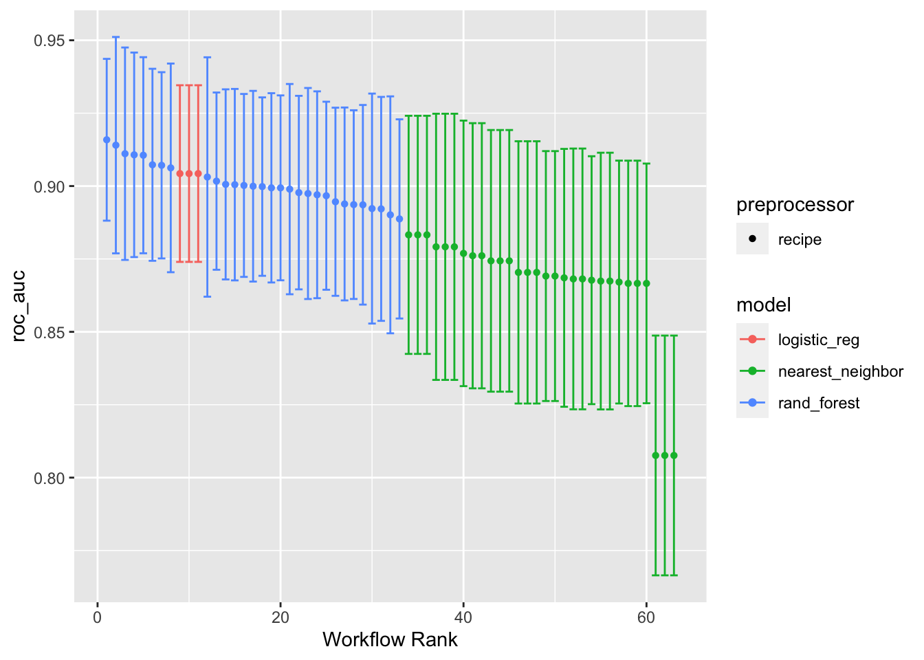
Adding select_best = TRUE will print out the best for each modeling algorithm. The default is to print the top three for each algorithm.
autoplot(models_tuned_wset, metric = "roc_auc", select_best = TRUE)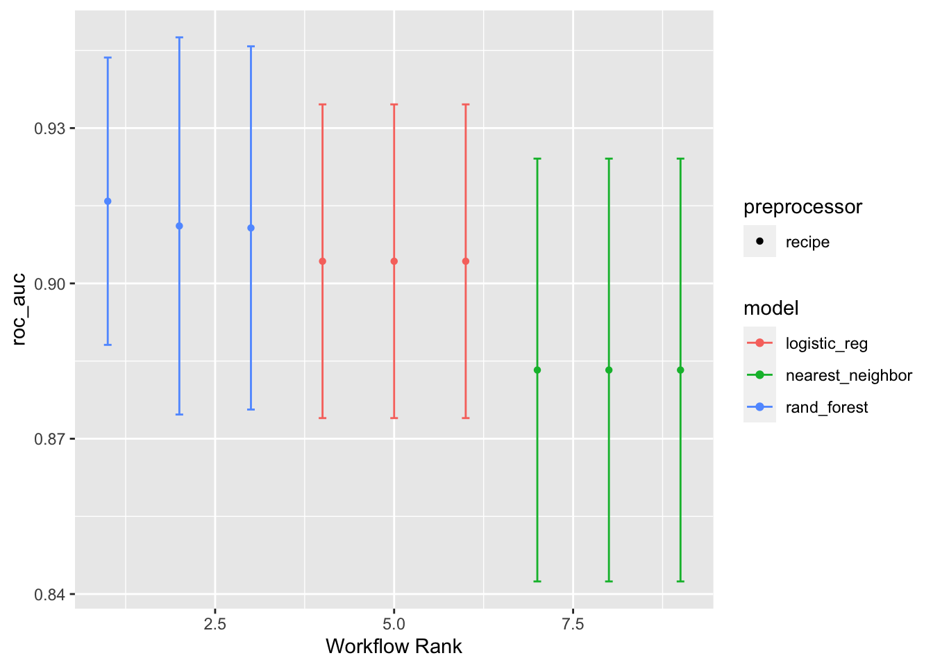
Final Model Selection
To select the final model, the tuned workflow_set() object can be passed to the rank_results() function. This function will rank models by the best mean performance metrics over the cross-validation folds. Setting the argument rank_metric = "roc_auc" ranks the models by the AUC. Setting the argument select_best = TRUE will return only the best models, rather than all of them.
models_tuned_wset %>%
  rank_results(rank_metric = "roc_auc", select_best = TRUE) %>%
  select(rank, mean, model, wflow_id, .config)
# A tibble: 9 × 5
rank mean model wflow_id .config
<int> <dbl> <chr> <chr> <chr>
1 1 0.916 rand_forest recipe_1_rand_forest Preprocessor1_Model04
2 2 0.911 rand_forest recipe_3_rand_forest Preprocessor1_Model07
3 3 0.911 rand_forest recipe_2_rand_forest Preprocessor1_Model07
4 4 0.904 logistic_reg recipe_1_logistic_reg Preprocessor1_Model1
5 5 0.904 logistic_reg recipe_2_logistic_reg Preprocessor1_Model1
6 6 0.904 logistic_reg recipe_3_logistic_reg Preprocessor1_Model1
7 7 0.883 nearest_neighbor recipe_1_nearest_neighbor Preprocessor1_Model02
8 8 0.883 nearest_neighbor recipe_3_nearest_neighbor Preprocessor1_Model02
9 9 0.883 nearest_neighbor recipe_2_nearest_neighbor Preprocessor1_Model02To extract a specific model, the extract_workflow_set_result() can be used. The exact ID of the model can be specified with the id argument. This will return the cross-validation results for that specific model.
models_tuned_wset %>%
  extract_workflow_set_result(id = "recipe_1_rand_forest")
# Tuning results
# 10-fold cross-validation
# A tibble: 10 × 4
splits id .metrics .notes
<list> <chr> <list> <list>
1 <split [209/24]> Fold01 <tibble [10 × 7]> <tibble [0 × 3]>
2 <split [209/24]> Fold02 <tibble [10 × 7]> <tibble [0 × 3]>
3 <split [209/24]> Fold03 <tibble [10 × 7]> <tibble [0 × 3]>
4 <split [210/23]> Fold04 <tibble [10 × 7]> <tibble [0 × 3]>
5 <split [210/23]> Fold05 <tibble [10 × 7]> <tibble [0 × 3]>
6 <split [210/23]> Fold06 <tibble [10 × 7]> <tibble [0 × 3]>
7 <split [210/23]> Fold07 <tibble [10 × 7]> <tibble [0 × 3]>
8 <split [210/23]> Fold08 <tibble [10 × 7]> <tibble [0 × 3]>
9 <split [210/23]> Fold09 <tibble [10 × 7]> <tibble [0 × 3]>
10 <split [210/23]> Fold10 <tibble [10 × 7]> <tibble [0 × 3]>To extract the tuned hypearparameters of a specific model, pass the result of the extract_workflow_set_result() function into the select_best() function. Specifying the argument metric = "roc_auc" ensures that the combination of hyperparameters selected are the ones that, on average, maximized the AUC.
best_params_tbl <- models_tuned_wset %>%
  extract_workflow_set_result(id = "recipe_1_rand_forest") %>%
  select_best(metric = "roc_auc")

best_params_tbl
# A tibble: 1 × 4
mtry trees min_n .config
<int> <int> <int> <chr>
1 1 340 20 Preprocessor1_Model04Finally, the final model can be fit by passing the extracted workflow_set() of tuned models into the extract_workflow() function, specifying the ID of the desired model using the id argument. From there, this can be passed into the finalize_workflow() function along with the tibble of optimal parameters. This process is similar to that of a regular workflow(). Additional information can found in a previous post on the workflows package.
mod_final_spec_wflw <- models_tuned_wset %>%
  extract_workflow(id = "recipe_1_rand_forest") %>%
  finalize_workflow(best_params_tbl)

mod_final_spec_wflw
══ Workflow ════════════════════════════════════════════════════════════════════
Preprocessor: Recipe
Model: rand_forest()
── Preprocessor ────────────────────────────────────────────────────────────────
0 Recipe Steps
── Model ───────────────────────────────────────────────────────────────────────
Random Forest Model Specification (classification)
Main Arguments:
mtry = 1
trees = 340
min_n = 20
Engine-Specific Arguments:
importance = TRUE
Computational engine: randomForest This final workflow() specification can be passed to the fit() function to fit the model.
══ Workflow [trained] ══════════════════════════════════════════════════════════
Preprocessor: Recipe
Model: rand_forest()

── Preprocessor ────────────────────────────────────────────────────────────────
0 Recipe Steps

── Model ───────────────────────────────────────────────────────────────────────

Call:
 randomForest(x = maybe_data_frame(x), y = y, ntree = ~340L, mtry = min_cols(~1L,      x), nodesize = min_rows(~20L, x), importance = ~TRUE)
               Type of random forest: classification
                     Number of trees: 340
No. of variables tried at each split: 1

        OOB estimate of  error rate: 13.3%
Confusion matrix:
          Adelie Chinstrap class.error
Adelie       104        17   0.1404959
Chinstrap     14        98   0.1250000
Now that there is a final model, it can be used to make predictions. Among other methods, the augment() function can be used to calculate both probability and class predictions from the test data by passing in the final workflow() object and the test data. More information on the augment() function can be found in a previous post on the broom package.
mod_final_preds_tbl <- mod_final_fit_wflw %>%
  augment(penguins_test_tbl) %>%
  relocate(starts_with(".pred"), everything())

mod_final_preds_tbl
# A tibble: 100 × 10
.pred_class .pred_Adelie .pred_Chinstrap species island bill_length_mm
<fct> <dbl> <dbl> <fct> <fct> <dbl>
1 Chinstrap 0.15 0.85 Chinstrap Torgersen 40.3
2 Adelie 0.918 0.0824 Adelie Torgersen 39.2
3 Chinstrap 0.229 0.771 Chinstrap Torgersen 38.7
4 Adelie 0.885 0.115 Adelie Torgersen 46
5 Chinstrap 0.0971 0.903 Chinstrap Biscoe 37.8
6 Adelie 0.629 0.371 Adelie Biscoe 37.7
7 Adelie 0.815 0.185 Adelie Biscoe 38.2
8 Adelie 0.788 0.212 Chinstrap Biscoe 40.6
9 Chinstrap 0.0294 0.971 Chinstrap Dream 36.4
10 Chinstrap 0.291 0.709 Adelie Dream 42.2
# ℹ 90 more rows
# ℹ 4 more variables: bill_depth_mm <dbl>, flipper_length_mm <int>,
# body_mass_g <int>, sex <fct>Out-of-sample performance on the test data can be calculated using functions such as conf_mat(), for the confusion matrix, and roc_auc(), for the AUC, by passing in the test data predictions. Overall, it would seem that this final model does a good job at predicting out-of-sample data due to its large AUC and relatively few incorrectly classified outcome classes.
Notes
This post is based on a presentation that was given on the date listed. It may be updated from time to time to fix errors, detail new functions, and/or remove deprecated functions so the packages and R version will likely be newer than what was available at the time.
The R session information used for this post:
R version 4.2.1 (2022-06-23)
Platform: aarch64-apple-darwin20 (64-bit)
Running under: macOS 14.1.1

Matrix products: default
BLAS:   /Library/Frameworks/R.framework/Versions/4.2-arm64/Resources/lib/libRblas.0.dylib
LAPACK: /Library/Frameworks/R.framework/Versions/4.2-arm64/Resources/lib/libRlapack.dylib

locale:
[1] en_US.UTF-8/en_US.UTF-8/en_US.UTF-8/C/en_US.UTF-8/en_US.UTF-8

attached base packages:
[1] stats     graphics  grDevices datasets  utils     methods   base

other attached packages:
 [1] broom_1.0.5        workflows_1.1.2    yardstick_1.1.0    tune_1.1.2
 [5] dials_1.1.0        scales_1.2.1       parsnip_1.0.3      recipes_1.0.4
 [9] dplyr_1.1.3        rsample_1.2.0      workflowsets_1.0.1

loaded via a namespace (and not attached):
 [1] tidyr_1.3.0          jsonlite_1.8.0       splines_4.2.1
 [4] foreach_1.5.2        prodlim_2019.11.13   GPfit_1.0-8
 [7] renv_0.16.0          yaml_2.3.5           globals_0.16.2
[10] ipred_0.9-13         pillar_1.9.0         backports_1.4.1
[13] lattice_0.20-45      glue_1.6.2           digest_0.6.29
[16] randomForest_4.7-1.1 hardhat_1.2.0        colorspace_2.0-3
[19] htmltools_0.5.3      Matrix_1.4-1         timeDate_4022.108
[22] pkgconfig_2.0.3      lhs_1.1.6            DiceDesign_1.9
[25] listenv_0.8.0        purrr_1.0.2          gower_1.0.1
[28] lava_1.7.1           timechange_0.1.1     tibble_3.2.1
[31] farver_2.1.1         generics_0.1.3       ggplot2_3.4.0
[34] ellipsis_0.3.2       withr_2.5.1          furrr_0.3.1
[37] nnet_7.3-17          cli_3.6.1            survival_3.3-1
[40] magrittr_2.0.3       evaluate_0.16        fansi_1.0.4
[43] future_1.29.0        parallelly_1.32.1    MASS_7.3-57
[46] class_7.3-20         tools_4.2.1          lifecycle_1.0.3
[49] stringr_1.5.0        munsell_0.5.0        compiler_4.2.1
[52] rlang_1.1.1          grid_4.2.1           iterators_1.0.14
[55] rstudioapi_0.14      labeling_0.4.2       rmarkdown_2.16
[58] gtable_0.3.1         codetools_0.2-18     R6_2.5.1
[61] lubridate_1.9.0      knitr_1.40           fastmap_1.1.0
[64] future.apply_1.10.0  utf8_1.2.3           stringi_1.7.12
[67] parallel_4.2.1       Rcpp_1.0.9           vctrs_0.6.3
[70] rpart_4.1.19         tidyselect_1.2.0     xfun_0.40